How to Train a Flow Matching Image Generator From Scratch
I trained a flow matching image generation model from scratch on 21,551 anime faces. The model is unconditional, generates 64×64 images, and has 57 million trainable parameters.
“From scratch” needs one qualification: the flow model starts from random weights, but it operates in the latent space of a frozen FLUX.2/Ideogram-4 VAE. The VAE is the only pretrained component. This keeps the experiment focused on learning the generative flow rather than spending most of the compute on pixel reconstruction.
| Training metric | Result |
|---|---|
| Training images | 21,551 |
| Effective data with horizontal flips | 43,102 images |
| Trainable parameters | 57.0M |
| Training length | 10,000 epochs, about 210K optimizer steps |
| Final velocity cosine similarity | 0.670 |
| Final velocity magnitude ratio | 0.670 |
| VAE reconstruction PSNR | 26.9 dB |
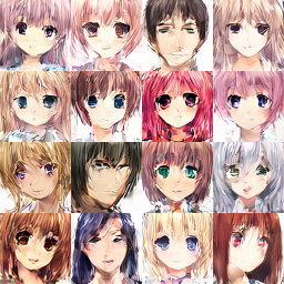
Final-checkpoint samples generated with EMA weights, Heun integration, and temperature 0.6.
# How Flow Matching Image Generation Works
Flow Matching learns a continuous velocity field that transports simple Gaussian noise into the data distribution. Unlike a diffusion model that predicts noise across a hand-designed noising process, this experiment used a straight path between noise and an image latent.
Let x₀ be Gaussian noise and x₁ be a real image latent. For a sampled time
t, the training point and target velocity are:
xₜ = (1 − t)x₀ + tx₁- target velocity:
u = x₁ − x₀ - loss:
L = mean((vθ(xₜ, t) − u)²)
The model predicts vθ, the direction and speed that should move the current
latent toward an image. I sampled t from a logit-normal distribution, following
the perceptually weighted rectified-flow recipe explored in
Stable Diffusion 3.
At inference time, generation starts from random noise and integrates
dx/dt = vθ(x,t) from t=0 to t=1. The final latent is then decoded into an
RGB image by the frozen VAE.
# A Small MLP Instead of a Diffusion Transformer
Each 64×64 image becomes an 8×8×32 VAE latent. I standardized the 32 channels, flattened the full latent into 2,048 values, and passed it through a residual SwiGLU MLP:
- hidden width: 768
- residual blocks: 8
- expansion ratio: 4
- time conditioning: sinusoidal embedding with AdaLN-Zero
- output: a velocity tensor with the same shape as the latent
There is no attention and no text conditioning. That makes the architecture easy to reason about: the network receives one flattened image state and a timestep, then predicts one velocity vector.
# The Training Recipe
The final run used a batch size of 1,024 and AdamW with a cosine learning-rate
schedule from 2e-4 to 1e-5. Four implementation choices mattered most:
- Cache VAE latents. Encode the dataset once so every training step works directly on small latent tensors.
- Pair noise and data with minibatch optimal transport. A chunked Hungarian assignment matches each image latent with nearby noise, making the paths straighter and the velocity target easier to learn.
- Use horizontal-flip augmentation. Caching both orientations doubled the effective dataset without adding work inside the VAE.
- Maintain exponential moving average weights. I used an EMA decay of
0.9999and sampled from the smoothed model rather than the noisier live weights.
Training ran on a single RTX A4500. Based on the checkpoint timestamps, the 10,000-epoch run took roughly three hours. At the recorded rental rate of $0.25/hour, the main training run cost less than one dollar.
# Sampling and Diagnostics
I used 50 ODE steps with Heun’s second-order method. It costs roughly twice as many velocity evaluations as Euler integration, but produces a more accurate trajectory without retraining the network.
The most useful diagnostic came from running the flow backward on real images.
The round trip reconstructed them at 46.75 dB PSNR, confirming that the learned
mapping was nearly reversible. However, the recovered noise had standard
deviation 0.589 rather than 1.0.
That measurement explained why sampling temperature mattered. Starting from
N(0, 0.6²) matched the region of noise space that the model had actually
associated with data and produced cleaner faces. Temperature 0.5–0.6 was the
best quality range, with the expected trade-off of lower diversity.
The VAE reconstruction score of 26.9 dB also showed that the latent codec was not the main bottleneck. The remaining softness and structural errors came primarily from the learned velocity field.
# A Practical Recipe
For a compact Flow Matching image generator, the reusable recipe is:
- encode images into a stable latent space and standardize its channels
- train the velocity field from random initialization with straight-path MSE
- use noise–data pairings and lightweight augmentation to make the transport problem easier
- keep exponential-moving-average weights for sampling
- use a second-order ODE solver such as Heun at inference time
- measure direction, magnitude calibration, sample quality, and reversibility instead of relying on loss alone
The core objective fits in a few equations. The engineering challenge is making the learned transport field cover the full data and noise distributions. A good latent space, well-conditioned paths, and explicit diagnostics do more for a small model than adding complexity without a measurement plan.